SciML Ecosystem

TAMIDS Workshop

Shao-Ting Chiu

Texas A&M Univ.

10/25/22

Scientific Machine Learning¹

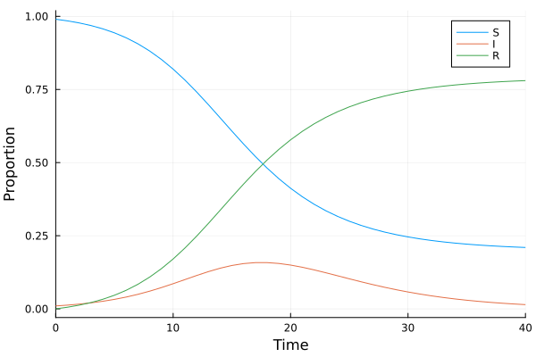
\[\begin{equation} u(t) = \begin{bmatrix} S(t)\\ I(t)\\ R(t) \end{bmatrix} \end{equation}\]

Machine Learning (Data-Driven)¹

\[\frac{du}{dt} = NN(u, p, t)\]

Physical Modeling

\[\frac{du}{dt} = f(u, p, t)\]

1. where \(NN(\cdot) \approx f(\cdot)\)

Scientific Machine Learning

Machine Learning (Data-Driven)

\[\frac{du}{dt} = NN(u, p, t)\]

NN = Chain(Dense(4,32,tanh),
           Dense(32,32,tanh),
           Dense(32,3))

Physical Modeling

\[\frac{du}{dt} = f(u, p, t)\]

function sir_ode(u,p,t)
    (S,I,R) = u
    (β,γ) = p
    dS = -β*S*I
    dI = β*S*I - γ*I
    dR = β*S*I
    [dS,dI,dR]
end;

	Data Driven	Physical Modeling
Pros	Universal approximation	Small training set, interpretation
Cons	Requires tremendous data	Requires analytical expression

• The question is
  • How to combine two separated ecosystems into unified high-performance framework.

SciML Software

• An Open Source Software for Scientific Machine Learning ¹
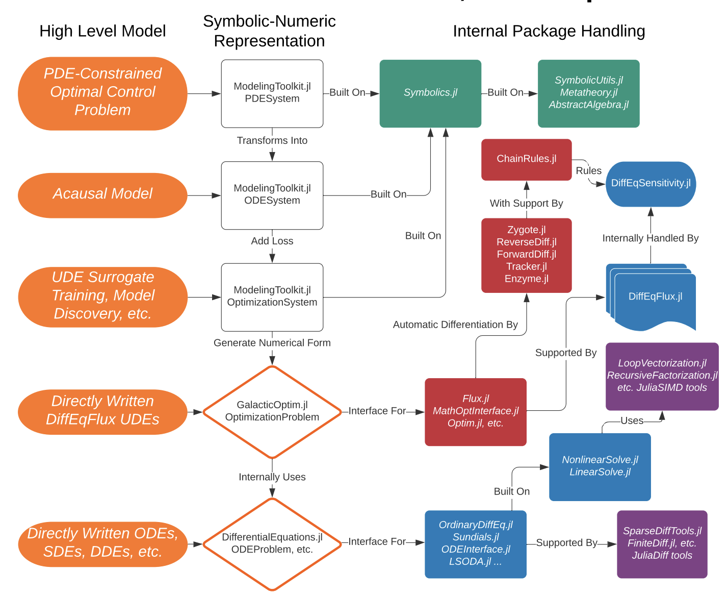
• Leverage the type inference and multiple dispatche of Julia to integrate packages.
• This ecosystem supports
  1. Differential Equation Solving
     • DifferentialEquations.jl
  2. Physics-informed model discovery
     • DiffEqFlux.jl
  3. Parameter Estimation and Bayesian Analysis
     • DataDrivenDiffEq.jl
  4. And many others (134 packages in total)

1. https://sciml.ai/

SciML Software¹

1. Image is from Figure 1. of Rackauckas, Christopher, et al. “Universal differential equations for scientific machine learning.” arXiv preprint arXiv:2001.04385 (2020).

Example

Suppose we have a ground truth model \(u(t) = [S(t), I(t), C(t)]^T\)

\[\begin{align} \frac{dS}{dt} &= -\beta S(t)I(t)\\ \frac{dI}{dt} &= \beta S(t)I(t)-\gamma I(t)\\ \frac{dR}{dt} &= \beta S(t)I(t) \end{align}\]

where \(\beta\) and \(\gamma\) are nonnegative parameters.

Data and Prior knowledge

• Data: \(\{u(t), t\}\)

• Model with unknown mechanism \(\lambda: R^3\to R\). Such that \[\begin{align} \frac{dS}{dt} &= -\lambda(I(t), \beta, \gamma) S(t)\\ \frac{dI}{dt} &= \lambda(I(t), \beta, \gamma) S(t)-\gamma I(t)\\ \frac{dR}{dt} &= \lambda(I(t), \beta, \gamma)S(t) \end{align}\]

• Also, let \(\lambda\) be the approximated function of a part of the truth model

Use Convolutional Neural Network for surrogation

• By universal approximation theorem,

\[\begin{align} \frac{dS}{dt} &= -\lambda_{NN}(I(t), \beta, \gamma) S(t)\\ \frac{dI}{dt} &= \lambda_{NN}(I(t), \beta, \gamma) S(t)-\gamma I(t)\\ \frac{dR}{dt} &= \lambda_{NN}(I(t), \beta, \gamma)S(t) \end{align}\]

• This is the universal ordinary differential equation²

Implementation

Universal Differential Equation (UDE)

\[\begin{align} \frac{dS}{dt} &= -\lambda_{NN}(I(t), \beta, \gamma) S(t)\\ \frac{dI}{dt} &= \lambda_{NN}(I(t), \beta, \gamma) S(t)-\gamma I(t)\\ \frac{dR}{dt} &= \lambda_{NN}(I(t), \beta, \gamma)S(t) \end{align}\]

Implementation

function sir_ude(u,p_,t,foi, st)
    # Current State
    S,I,C = u
    β,γ = p
    # CNN
    λ= foi([I], p_, st)[1][1] 
    # UDE
    dS = -λ*S
    dI = λ*S - γ*I
    dR = λ*S
    [dS, dI, dR]
end;

• To achieve this task, integration of multiple frameworks is necessary.

Tasks	SciML Package
ODE solver	DifferentialEquations.jl
Neural network	Flux.jl/Lux.jl
Differential programming	Zygote.jl
Optimization	Optimization.jl

Model Discovery and why we need it?

• Suppose the UDE¹ model is successfully fitted with dataset \(\{u(t), t\}\)

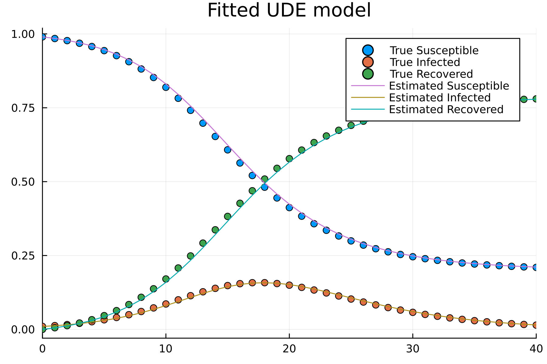
\[\begin{align} \frac{dS}{dt} &= -\lambda_{NN}(I(t), \beta, \gamma) S(t)\\ \frac{dI}{dt} &= \lambda_{NN}(I(t), \beta, \gamma) S(t)-\gamma I(t)\\ \frac{dR}{dt} &= \lambda_{NN}(I(t), \beta, \gamma)S(t) \end{align}\]

• How is the extrapolation?
  • Such as \(u_{ext}(t_{ext}) \notin \{u(t), t\}\)

1. Universal Ordinary Differential Equation²

Model Discovery and why we need it?

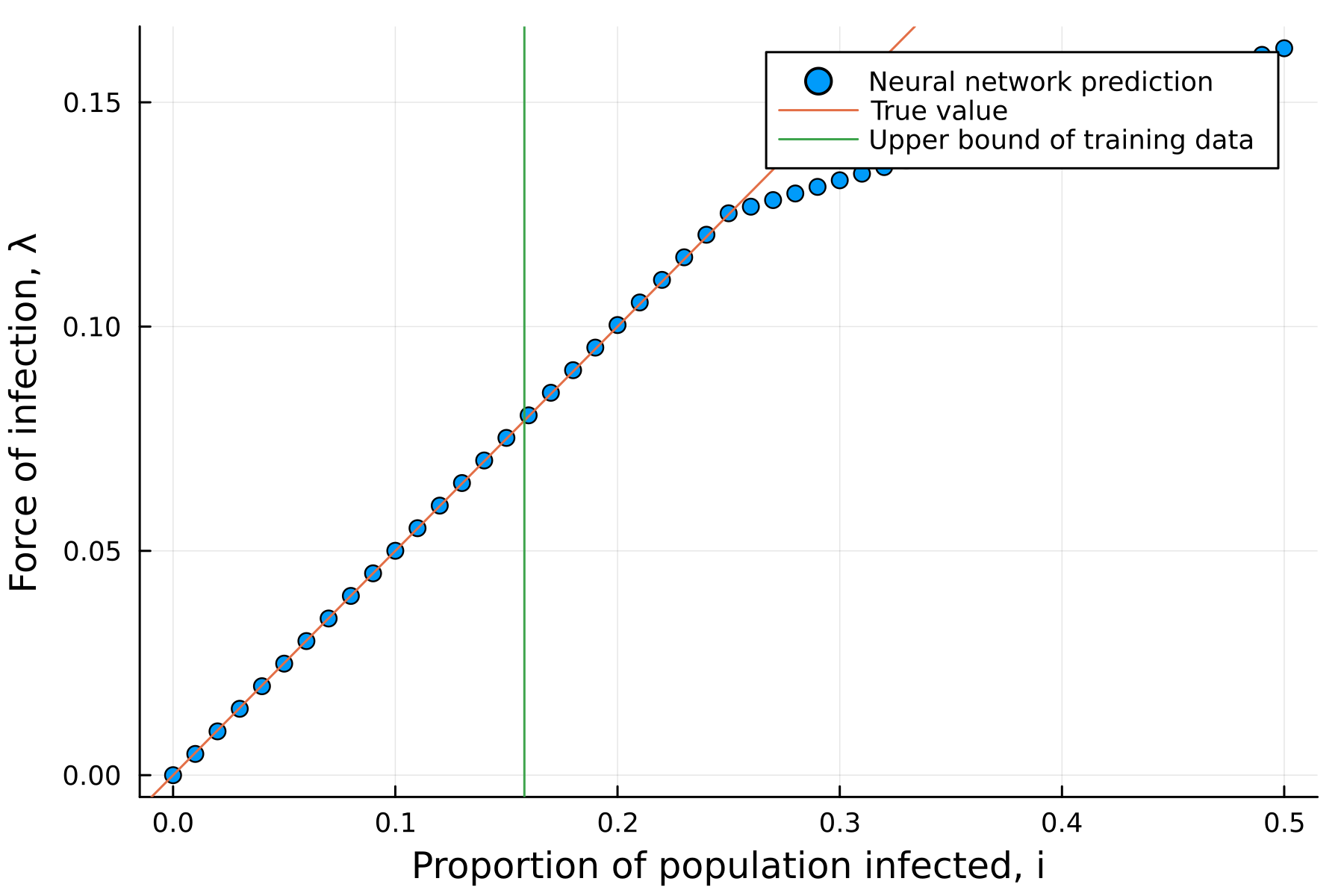
• We should get

\[\lambda_{NN}(I, \beta, \gamma) \approx \beta I\]

• However, the extrapolation of nerual network is errornous.
• Sparsification of neural networks is needed (Occam’s razor).
  • Symbolic regressions¹
  • DataDrivenDiffEq.jl

1. Such as sparse identification³

Application and Industry¹

• Cedar\(^{\text{EDA}}\): differentiable analog circuit with machine learning
  • SPICE (C++)
• Pumas-AI: Model-informed drug development with machine learning
  • NONMEM (Fortran)
• Macroeconomics, climate, urban development

1. more cases are on https://juliacomputing.com/case-studies/

Remarks

1. Julia provides great compiler design for the extensiblity.
2. With the state-out-art compiler design, many impactful application starts to outcompete old methods.
3. Writing high-level script with efficient performance is the key feature of using Julia.

Hands-on session

• Julia basics
• UDE example

References

1.

Baker, N., Alexander, F., Bremer, T., Hagberg, A., Kevrekidis, Y., Najm, H., Parashar, M., Patra, A., Sethian, J., Wild, S., et al. (2019). Workshop Report on Basic Research Needs for Scientific Machine Learning: Core Technologies for Artificial Intelligence 10.2172/1478744.

2.

Rackauckas, C., Ma, Y., Martensen, J., Warner, C., Zubov, K., Supekar, R., Skinner, D., Ramadhan, A., and Edelman, A. (2020). Universal differential equations for scientific machine learning. arXiv preprint arXiv:2001.04385.

3.

Brunton, S.L., Proctor, J.L., and Kutz, J.N. (2016). Discovering governing equations from data by sparse identification of nonlinear dynamical systems. Proceedings of the national academy of sciences 113, 3932–3937.