SciML Ecosystem

Presentation

• Slides

Scientific Machine Learning [1]

\[\begin{equation} u(t) = \begin{bmatrix} S(t)\\ I(t)\\ R(t) \end{bmatrix} \end{equation}\]

Machine Learning (Data-Driven)¹

\[\frac{du}{dt} = NN(u, p, t)\]

Physical Modeling

\[\frac{du}{dt} = f(u, p, t)\]

---

Scientific Machine Learning

Machine Learning (Data-Driven)

\[\frac{du}{dt} = NN(u, p, t)\]

NN = Chain(Dense(4,32,tanh),
           Dense(32,32,tanh),
           Dense(32,3))

Physical Modeling

\[\frac{du}{dt} = f(u, p, t)\]

function sir_ode(u,p,t)
    (S,I,R) = u
    (β,γ) = p
    dS = -β*S*I
    dI = β*S*I - γ*I
    dR = β*S*I
    [dS,dI,dR]
end;

	Data Driven	Physical Modeling
Pros	Universal approximation	Small training set, interpretation
Cons	Requires tremendous data	Requires analytical expression

• The question is
  • How to combine two separated ecosystems into unified high-performance framework.

---

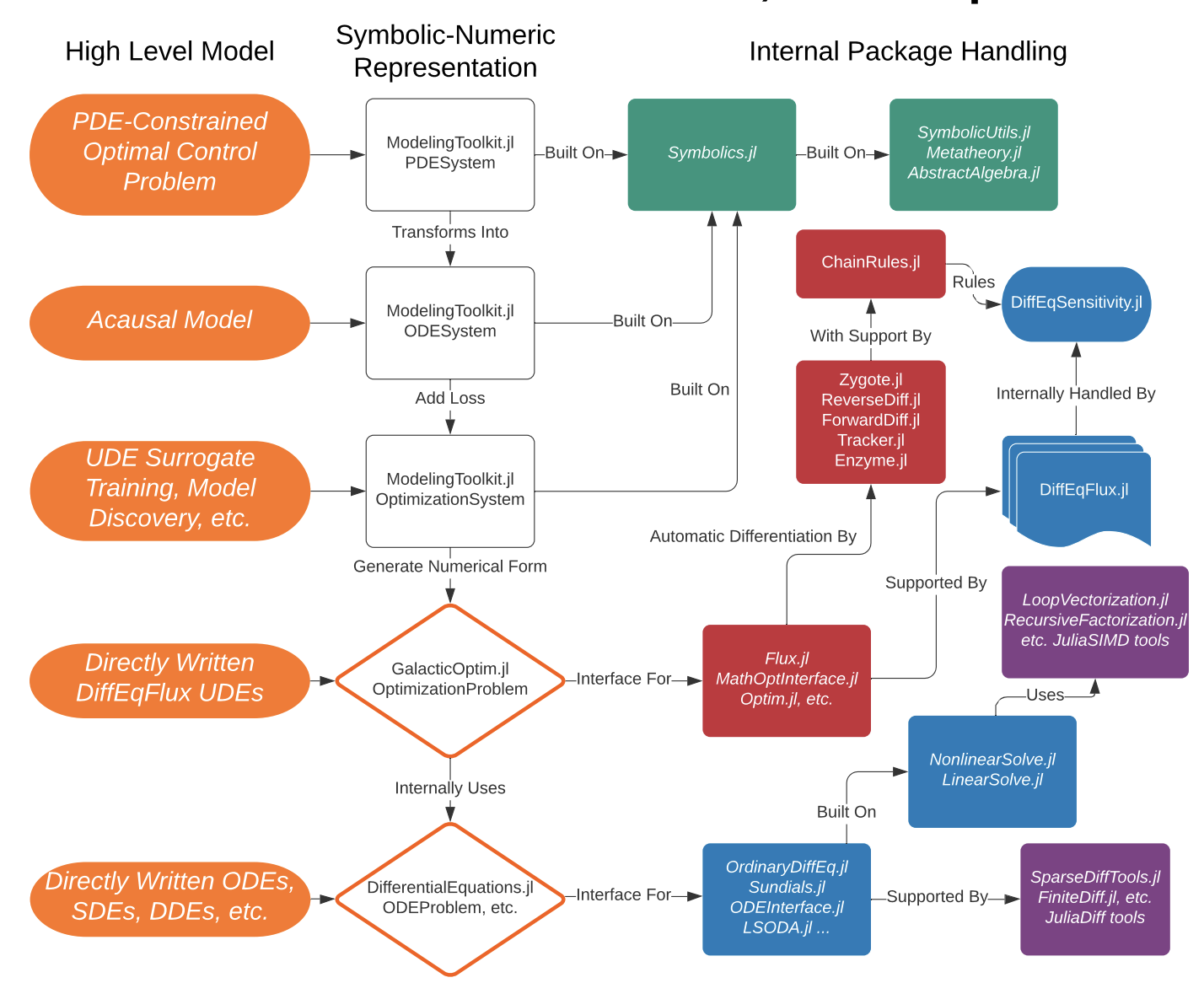
SciML Software

• An Open Source Software for Scientific Machine Learning ²
• Leverage the type inference and multiple dispatche of Julia to integrate packages.
• This ecosystem supports
  1. Differential Equation Solving
     • DifferentialEquations.jl
  2. Physics-informed model discovery
     • DiffEqFlux.jl
  3. Parameter Estimation and Bayesian Analysis
     • DataDrivenDiffEq.jl
  4. And many others (134 packages in total)

---

SciML Software³

---

Example

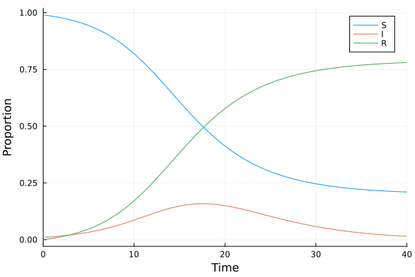
Suppose we have a ground truth model \(u(t) = [S(t), I(t), C(t)]^T\)

\[\begin{align} \frac{dS}{dt} &= -\beta S(t)I(t)\\ \frac{dI}{dt} &= \beta S(t)I(t)-\gamma I(t)\\ \frac{dR}{dt} &= \beta S(t)I(t) \end{align}\]

where \(\beta\) and \(\gamma\) are nonnegative parameters.

---

Data and Prior knowledge

• Data: \(\{u(t), t\}\)

• Model with unknown mechanism \(\lambda: R^3\to R\). Such that \[\begin{align} \frac{dS}{dt} &= -\lambda(I(t), \beta, \gamma) S(t)\\ \frac{dI}{dt} &= \lambda(I(t), \beta, \gamma) S(t)-\gamma I(t)\\ \frac{dR}{dt} &= \lambda(I(t), \beta, \gamma)S(t) \end{align}\]

• Also, let \(\lambda\) be the approximated function of a part of the truth model

---

Use Convolutional Neural Network for surrogation

• By universal approximation theorem,

\[\begin{align} \frac{dS}{dt} &= -\lambda_{NN}(I(t), \beta, \gamma) S(t)\\ \frac{dI}{dt} &= \lambda_{NN}(I(t), \beta, \gamma) S(t)-\gamma I(t)\\ \frac{dR}{dt} &= \lambda_{NN}(I(t), \beta, \gamma)S(t) \end{align}\]

• This is the universal ordinary differential equation[3]

---

Implementation

Universal Differential Equation (UDE)

\[\begin{align} \frac{dS}{dt} &= -\lambda_{NN}(I(t), \beta, \gamma) S(t)\\ \frac{dI}{dt} &= \lambda_{NN}(I(t), \beta, \gamma) S(t)-\gamma I(t)\\ \frac{dR}{dt} &= \lambda_{NN}(I(t), \beta, \gamma)S(t) \end{align}\]

Implementation

function sir_ude(u,p_,t,foi, st)
    # Current State
    S,I,C = u
    β,γ = p
    # CNN
    λ= foi([I], p_, st)[1][1] 
    # UDE
    dS = -λ*S
    dI = λ*S - γ*I
    dR = λ*S
    [dS, dI, dR]
end;

• To achieve this task, integration of multiple frameworks is necessary.

Tasks	SciML Package
ODE solver	DifferentialEquations.jl
Neural network	Flux.jl/Lux.jl
Differential programming	Zygote.jl
Optimization	Optimization.jl

---

Model Discovery and why we need it?

• Suppose the UDE⁴ model is successfully fitted with dataset \(\{u(t), t\}\)

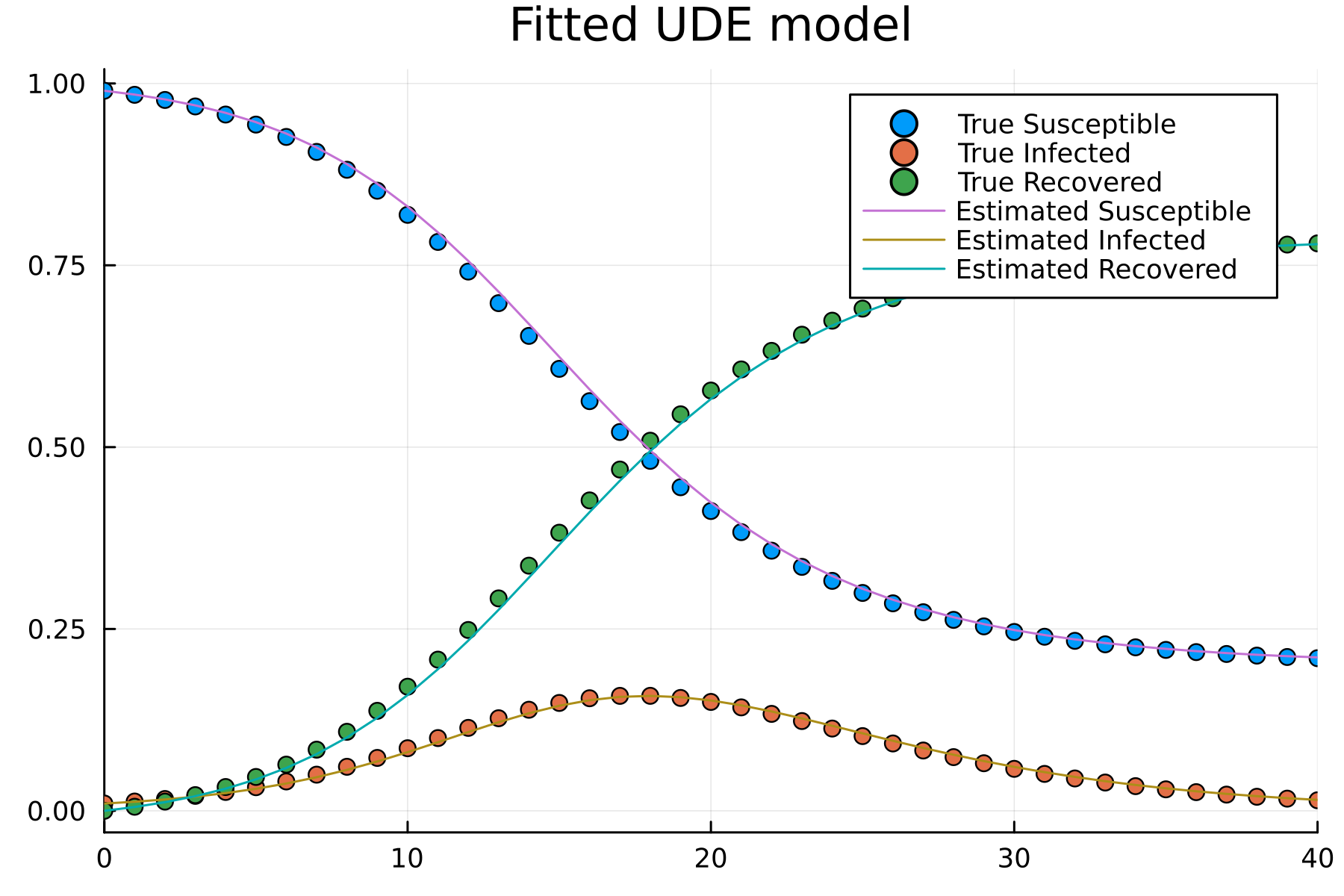
\[\begin{align} \frac{dS}{dt} &= -\lambda_{NN}(I(t), \beta, \gamma) S(t)\\ \frac{dI}{dt} &= \lambda_{NN}(I(t), \beta, \gamma) S(t)-\gamma I(t)\\ \frac{dR}{dt} &= \lambda_{NN}(I(t), \beta, \gamma)S(t) \end{align}\]

• How is the extrapolation?
  • Such as \(u_{ext}(t_{ext}) \notin \{u(t), t\}\)

---

Model Discovery and why we need it?

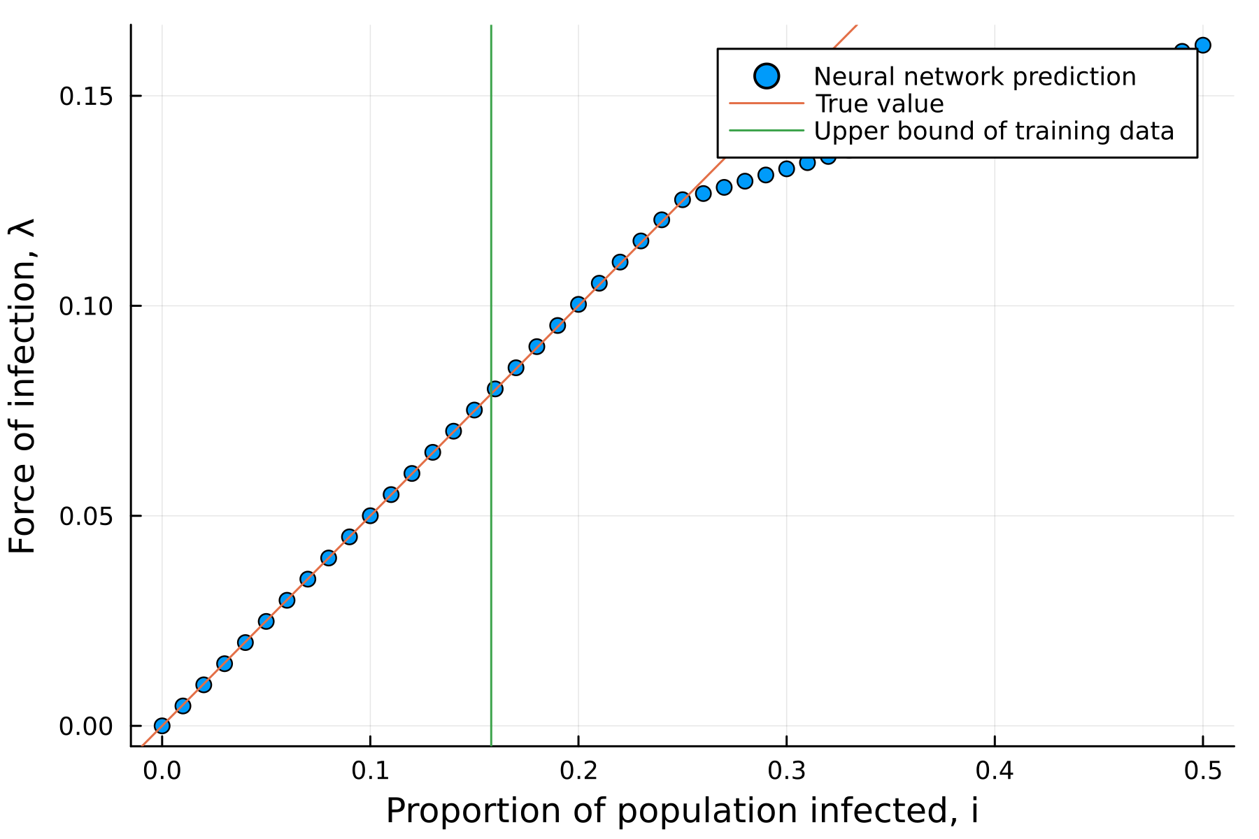
• We should get

\[\lambda_{NN}(I, \beta, \gamma) \approx \beta I\]

• However, the extrapolation of nerual network is errornous.
• Sparsification of neural networks is needed (Occam’s razor).
  • Symbolic regressions⁵
  • DataDrivenDiffEq.jl

---

Application and Industry⁶

• Cedar\(^{\text{EDA}}\): differentiable analog circuit with machine learning
  • SPICE (C++)
• Pumas-AI: Model-informed drug development with machine learning
  • NONMEM (Fortran)
• Macroeconomics, climate, urban development

---

Remarks

1. Julia provides great compiler design for the extensiblity.
2. With the state-out-art compiler design, many impactful application starts to outcompete old methods.
3. Writing high-level script with efficient performance is the key feature of using Julia.

---

Hands-on session

• Julia basics
• UDE example

---

References

[1]

Baker, N. et al. 2019. Workshop Report on Basic Research Needs for Scientific Machine Learning: Core Technologies for Artificial Intelligence. Technical Report #1478744.

[2]

Brunton, S.L. et al. 2016. Discovering governing equations from data by sparse identification of nonlinear dynamical systems. Proceedings of the national academy of sciences. 113, 15 (2016), 3932–3937.

[3]

Rackauckas, C. et al. 2020. Universal differential equations for scientific machine learning. arXiv preprint arXiv:2001.04385. (2020).

Footnotes

1. where \(NN(\cdot) \approx f(\cdot)\)

2. https://sciml.ai/

3. Image is from Figure 1. of Rackauckas, Christopher, et al. “Universal differential equations for scientific machine learning.” arXiv preprint arXiv:2001.04385 (2020).

4. Universal Ordinary Differential Equation [3]

5. Such as sparse identification[2]

6. more cases are on https://juliacomputing.com/case-studies/