13  Predicting Stock Market with Bayesian Nerual Network

13.1 Fit sliding window of stock markets

13.2 Installing packages

!pip install git+https://github.com/deepmind/dm-haiku
!pip install git+https://github.com/jamesvuc/jax-bayes
Looking in indexes: https://pypi.org/simple, https://us-python.pkg.dev/colab-wheels/public/simple/
Collecting git+https://github.com/deepmind/dm-haiku
  Cloning https://github.com/deepmind/dm-haiku to /tmp/pip-req-build-roptddu5
  Running command git clone -q https://github.com/deepmind/dm-haiku /tmp/pip-req-build-roptddu5
Requirement already satisfied: absl-py>=0.7.1 in /usr/local/lib/python3.8/dist-packages (from dm-haiku==0.0.10.dev0) (1.3.0)
Collecting jmp>=0.0.2
  Downloading jmp-0.0.2-py3-none-any.whl (16 kB)
Requirement already satisfied: numpy>=1.18.0 in /usr/local/lib/python3.8/dist-packages (from dm-haiku==0.0.10.dev0) (1.21.6)
Requirement already satisfied: tabulate>=0.8.9 in /usr/local/lib/python3.8/dist-packages (from dm-haiku==0.0.10.dev0) (0.8.10)
Building wheels for collected packages: dm-haiku
  Building wheel for dm-haiku (setup.py) ... done
  Created wheel for dm-haiku: filename=dm_haiku-0.0.10.dev0-py3-none-any.whl size=614395 sha256=25abd727928e5aaeeeafa7caad835333acf006ea394957d67ececb647c2b4ee0
  Stored in directory: /tmp/pip-ephem-wheel-cache-idhjkii0/wheels/c7/4d/89/b159f184ad7c9e95672c342eafcc176ad92ee0c77f27f3bd23
Successfully built dm-haiku
Installing collected packages: jmp, dm-haiku
Successfully installed dm-haiku-0.0.10.dev0 jmp-0.0.2
Looking in indexes: https://pypi.org/simple, https://us-python.pkg.dev/colab-wheels/public/simple/
Collecting git+https://github.com/jamesvuc/jax-bayes
  Cloning https://github.com/jamesvuc/jax-bayes to /tmp/pip-req-build-n2yx3bkn
  Running command git clone -q https://github.com/jamesvuc/jax-bayes /tmp/pip-req-build-n2yx3bkn
Requirement already satisfied: absl-py>=0.9.0 in /usr/local/lib/python3.8/dist-packages (from jax-bayes==0.1.1) (1.3.0)
Requirement already satisfied: numpy>=1.18.0 in /usr/local/lib/python3.8/dist-packages (from jax-bayes==0.1.1) (1.21.6)
Requirement already satisfied: opt-einsum>=3.3.0 in /usr/local/lib/python3.8/dist-packages (from jax-bayes==0.1.1) (3.3.0)
Requirement already satisfied: protobuf>=3.12.4 in /usr/local/lib/python3.8/dist-packages (from jax-bayes==0.1.1) (3.19.6)
Requirement already satisfied: scipy>=1.5.2 in /usr/local/lib/python3.8/dist-packages (from jax-bayes==0.1.1) (1.7.3)
Requirement already satisfied: six>=1.15.0 in /usr/local/lib/python3.8/dist-packages (from jax-bayes==0.1.1) (1.15.0)
Requirement already satisfied: tqdm>=4.48.2 in /usr/local/lib/python3.8/dist-packages (from jax-bayes==0.1.1) (4.64.1)
Building wheels for collected packages: jax-bayes
  Building wheel for jax-bayes (setup.py) ... done
  Created wheel for jax-bayes: filename=jax_bayes-0.1.1-py3-none-any.whl size=1031680 sha256=9b907924ffc39bb28cbc9fc15f6fa0ae4fe85463be7b70cd798b52802fc3c4d7
  Stored in directory: /tmp/pip-ephem-wheel-cache-xyinnglr/wheels/3f/7b/9c/326882f09afedfadf20a391de383da7aaea36b633d5e17555f
Successfully built jax-bayes
Installing collected packages: jax-bayes
Successfully installed jax-bayes-0.1.1
13.3 Downloading data

!git clone https://github.com/stevengogogo/Bayesianneuralnet_stockmarket
Cloning into 'Bayesianneuralnet_stockmarket'...
remote: Enumerating objects: 960, done.
remote: Counting objects: 100% (10/10), done.
remote: Compressing objects: 100% (8/8), done.
remote: Total 960 (delta 3), reused 8 (delta 2), pack-reused 950
Receiving objects: 100% (960/960), 217.92 MiB | 15.57 MiB/s, done.
Resolving deltas: 100% (167/167), done.

13.4 Training Experiment

import os
import os.path as osp
import numpy as np
# %%
import numpy as np
np.random.seed(0)

import haiku as hk
import pandas as pd
import jax.numpy as jnp
import jax

from tqdm import tqdm, trange
from matplotlib import pyplot as plt

from jax_bayes.utils import confidence_bands
from jax_bayes.mcmc import (
     langevin_fns,
    mala_fns,
     hmc_fns,
)

13.5 Computational Devices

jax.devices()
[StreamExecutorGpuDevice(id=0, process_index=0, slice_index=0)]

13.6 Data processing

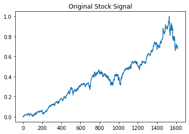
The original data set is \(x_t = \{x_{1}, ..., x_{Total}\}\), the training input is a matrix with dimension \(m \times s\) (where m is the capture window, and \(s\) is the number of samples). The sample is produced by shifting the original time series with lag of \(2\).

  • Training set

\[\bar{x}_t = \underbrace{\begin{bmatrix} x_{1+(t-1)T} & \cdots & x_{m+(t-1)T}\\ x_{3+(t-1)T} & \cdots & x_{2m+3+(t-1)T}\\ \vdots & \vdots & \vdots \end{bmatrix}}_{\text{m(Capture windows)}} \]

\[y_t = \underbrace{\begin{bmatrix} x_{m+(t-1)T + 1} & \cdots & x_{m+(t-1)T+ n}\\ x_{2m+3+(t-1)T + 1} & \cdots & x_{2m+3+(t-1)T+ n}\\ \vdots & \vdots & \vdots \end{bmatrix}}_{\text{n (Prediction Horizons)}} \]

  • \(m\): embedding dimension (predicting horizon)
  • \(T\): time lag
data_path_base = 'Bayesianneuralnet_stockmarket/code/datasets'

def get_orig(sig, shift=2):
    return np.concatenate((sig[0,:].ravel(), sig[1:,-shift:].ravel()))
    

# horizon
timesteps = 5
steps_ahead = 5

# load
train = np.loadtxt(open(os.path.join(data_path_base, "MMM8_train.txt")))
train.shape
(804, 10)
pd.DataFrame(train)
0 1 2 3 4 5 6 7 8 9
0 0.000554 0.003739 0.001985 0.000000 0.002308 0.004293 0.001846 0.004200 0.001062 0.003970
1 0.001985 0.000000 0.002308 0.004293 0.001846 0.004200 0.001062 0.003970 0.007847 0.011216
2 0.002308 0.004293 0.001846 0.004200 0.001062 0.003970 0.007847 0.011216 0.010524 0.010339
3 0.001846 0.004200 0.001062 0.003970 0.007847 0.011216 0.010524 0.010339 0.011816 0.014355
4 0.001062 0.003970 0.007847 0.011216 0.010524 0.010339 0.011816 0.014355 0.019432 0.018879
... ... ... ... ... ... ... ... ... ... ...
799 0.719476 0.720176 0.723407 0.705364 0.693515 0.701704 0.694112 0.709296 0.694166 0.692539
800 0.723407 0.705364 0.693515 0.701704 0.694112 0.709296 0.694166 0.692539 0.696552 0.694491
801 0.693515 0.701704 0.694112 0.709296 0.694166 0.692539 0.696552 0.694491 0.676650 0.692593
802 0.694112 0.709296 0.694166 0.692539 0.696552 0.694491 0.676650 0.692593 0.684730 0.697528
803 0.694166 0.692539 0.696552 0.694491 0.676650 0.692593 0.684730 0.697528 0.705500 0.706259

804 rows × 10 columns

# original time-series
orig = get_orig(train)

pd.DataFrame(orig[0:13])
0
0 0.000554
1 0.003739
2 0.001985
3 0.000000
4 0.002308
5 0.004293
6 0.001846
7 0.004200
8 0.001062
9 0.003970
10 0.007847
11 0.011216
12 0.010524
plt.plot(orig)
plt.title("Original Stock Signal");

train.shape
(804, 10)
x_train = train[:, :timesteps]
y_train = train[:, timesteps: timesteps + steps_ahead]
xy_train = (x_train, y_train)
pd.DataFrame(x_train)
0 1 2 3 4
0 0.000554 0.003739 0.001985 0.000000 0.002308
1 0.001985 0.000000 0.002308 0.004293 0.001846
2 0.002308 0.004293 0.001846 0.004200 0.001062
3 0.001846 0.004200 0.001062 0.003970 0.007847
4 0.001062 0.003970 0.007847 0.011216 0.010524
... ... ... ... ... ...
799 0.719476 0.720176 0.723407 0.705364 0.693515
800 0.723407 0.705364 0.693515 0.701704 0.694112
801 0.693515 0.701704 0.694112 0.709296 0.694166
802 0.694112 0.709296 0.694166 0.692539 0.696552
803 0.694166 0.692539 0.696552 0.694491 0.676650

804 rows × 5 columns

pd.DataFrame(y_train)
0 1 2 3 4
0 0.004293 0.001846 0.004200 0.001062 0.003970
1 0.004200 0.001062 0.003970 0.007847 0.011216
2 0.003970 0.007847 0.011216 0.010524 0.010339
3 0.011216 0.010524 0.010339 0.011816 0.014355
4 0.010339 0.011816 0.014355 0.019432 0.018879
... ... ... ... ... ...
799 0.701704 0.694112 0.709296 0.694166 0.692539
800 0.709296 0.694166 0.692539 0.696552 0.694491
801 0.692539 0.696552 0.694491 0.676650 0.692593
802 0.694491 0.676650 0.692593 0.684730 0.697528
803 0.692593 0.684730 0.697528 0.705500 0.706259

804 rows × 5 columns

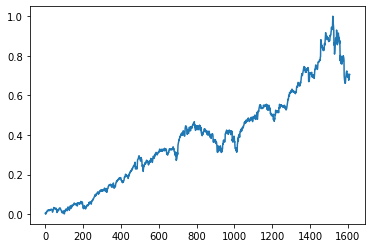
plt.plot(get_orig(y_train))

x_train.shape
(804, 5)
y_train.shape
(804, 5)
## BNN training

#could use any of the samplers modulo hyperparameters
# sampler_fns = hmc_fns
sampler_fns = langevin_fns
#sampler_fns = mala_fns


def net_fn(x):

    mlp = hk.Sequential([
        hk.Linear(128, w_init=hk.initializers.Constant(0), 
                       b_init=hk.initializers.Constant(0)), 
        jnp.tanh, 
        hk.Linear(5,   w_init=hk.initializers.Constant(0), 
                       b_init=hk.initializers.Constant(0))
        ])

    return mlp(x)
lr = 1e-4
reg = 0.1
lik_var = 0.5

net = hk.transform(net_fn)
key = jax.random.PRNGKey(0)

sampler_init, sampler_propose, sampler_accept, sampler_update, sampler_get_params = \
    sampler_fns(key, num_samples=30, step_size=lr, init_stddev=5.0)
def logprob(params, xy):
    """ log posterior, assuming 
    P(params) ~ N(0,eta)
    P(y|x, params) ~ N(f(x;params), lik_var)
    """
    x, y = xy

    preds = net.apply(params, None, x)
    log_prior = - reg * sum(jnp.sum(jnp.square(p)) 
                        for p in jax.tree_leaves(params))
    log_lik = - jnp.mean(jnp.square(preds - y)) / lik_var
    return log_lik + log_prior

@jax.jit
def sampler_step(i, state, keys, batch):
    # print(state)
    # input()
    params = sampler_get_params(state)
    logp = lambda params:logprob(params, batch)
    fx, dx = jax.vmap(jax.value_and_grad(logp))(params)

    fx_prop, dx_prop = fx, dx
    # fx_prop, prop_state, dx_prop, new_keys = fx, state, dx, keys
    prop_state, keys = sampler_propose(i, dx, state, keys)

    # for RK-langevin and MALA --- recompute gradients
    #prop_params = sampler_get_params(prop_state)
    #fx_prop, dx_prop = jax.vmap(jax.value_and_grad(logp))(prop_params)

    # for HMC
    prop_state, dx_prop, keys = state, dx, keys
    for j in range(5): #5 iterations of the leapfrog integrator
      prop_state, keys = \
      sampler_propose(i, dx_prop, prop_state, keys)

      prop_params = sampler_get_params(prop_state)
      fx_prop, dx_prop = jax.vmap(jax.value_and_grad(logp))(prop_params)

    accept_idxs, keys = sampler_accept(
        i, fx, fx_prop, dx, state, dx_prop, prop_state, keys
    )
    state, keys = sampler_update(
        i, accept_idxs, dx, state, dx_prop, prop_state, keys
    )


    return state, keys
# initialization
params = net.init(jax.random.PRNGKey(42), x_train)
sampler_state, sampler_keys = sampler_init(params)
/usr/local/lib/python3.8/dist-packages/haiku/_src/initializers.py:69: UserWarning: Explicitly requested dtype float64 requested in astype is not available, and will be truncated to dtype float32. To enable more dtypes, set the jax_enable_x64 configuration option or the JAX_ENABLE_X64 shell environment variable. See https://github.com/google/jax#current-gotchas for more.
  return jnp.broadcast_to(jnp.asarray(self.constant), shape).astype(dtype)
params['linear']['w'].shape
(5, 128)
#do the sampling
niter = 500000
train_logp = np.zeros(niter)
for step in trange(niter):
    # Training log
    sampler_params = sampler_get_params(sampler_state)
    logp = lambda params:logprob(params, xy_train)
    train_logp[step] = jnp.mean(jax.vmap(logp)(sampler_params))
    
    sampler_state, sampler_keys = \
        sampler_step(step, sampler_state, sampler_keys, xy_train)


sampler_params = sampler_get_params(sampler_state)
  0%|          | 0/500000 [00:00<?, ?it/s]FutureWarning: jax.tree_leaves is deprecated, and will be removed in a future release. Use jax.tree_util.tree_leaves instead.
  for p in jax.tree_leaves(params))
  2%|▏         | 8962/500000 [02:23<2:42:49, 50.26it/s]
# Training log
ftn, axtn = plt.subplots()
axtn.plot(train_logp[1000:])
axtn.set_xlabel("Iterations")
axtn.set_ylabel("Log likelihood")
#ftn.savefig("../img/training_MALA_{}-iter.pdf".format(niter))
outputs = jax.vmap(net.apply, in_axes=(0, None, None))(sampler_params, None, x_train)
outputs.shape
pred_lines = np.array([ get_orig(outputs[i,:,:]) for i in range(0, outputs.shape[0])])
pred_lines.shape
ms = jnp.mean(pred_lines, axis=0)
ss = jnp.std(pred_lines, axis=0)

lower, uper = ms-ss, ms+ss
x = jax.device_put(outputs)
fmma, axmma = plt.subplots()
axmma.plot(ms, label="Model average")
axmma.plot(orig, label="Ground truth")
for i in range(outputs.shape[0]):
        axmma.plot(get_orig(outputs[i,:,:]), color="gray",alpha=0.04)
axmma.set_xlabel("Time")
axmma.set_ylabel("A.U.")
axmma.set_title("MMM8 Prediction")
axmma.legend()
#fmma.savefig("../img/prediction_MALA_{}-iter.pdf".format(niter))
f, ax = plt.subplots(1)
for i in range(outputs.shape[0]):
        ax.plot(outputs[i,:,0], alpha=0.25)
ax.plot(ms, label="Mean")
ax.plot(y_train)
plt.plot(y_train[:,0])