4  Chapter 4: Monte Carlo Approximation

4.1 Mote Carlo Estimate

• Estimation of \(Var[\theta|y_1,\dots,y_n]\): \(\hat{\sigma}^2 = \sum \frac{(\theta^{(s)}\bar{\theta})^2}{S-1}\)
• Standard error: \(\sqrt{\frac{\hat{\sigma}^2}{S}}\)
• \(95\%\) Monte Carlo confidence interval: \(\hat{\theta} \pm 2 \sqrt{\frac{\hat{\sigma}^2}{S}}\)

\[std = \sqrt{\frac{\sigma^2}{n}}\]

4.2 Posterior inference for arbitrary functions

\[\log \text{odds}(\theta) = \log \frac{\theta}{1-\theta} = \gamma\]

#####   STAT 638
#### Matthias Katzfuss


#########   R code for Chapter 4   ##########


######   illustration of Monte Carlo for inverse rate in exponential

K=100000

## parameters of the posterior of the rate parameter
a=50
b=37815

## posterior draws of the rate parameter
theta=rgamma(K,a,rate=b)

## transform to mean parameter
psi=1/theta


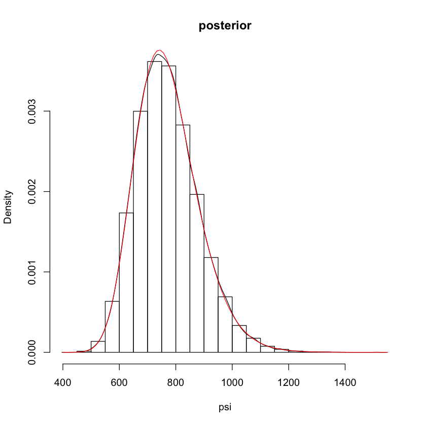
## plot posterior of psi
hist(psi,freq=FALSE,main='posterior') # histogram of psi draws
lines(density(psi)) # kernel-density estimate
curve(invgamma::dinvgamma(x,a,b),add=TRUE,col=2) # exact


## posterior mean
b/(a-1) # exact
mean(psi) # monte carlo approximation


## the larger K, the closer MC estimate 
##   *tends* to be to exact summary
plot(cumsum(psi)/(1:K),xlim=c(1,1000),type='l',
     xlab='K',ylab='MC mean based on K samples')
abline(h=b/(a-1),col='red')


## posterior standard deviation
sqrt(b^2/(a-1)^2/(a-2)) # exact
sd(psi) # monte carlo approximation


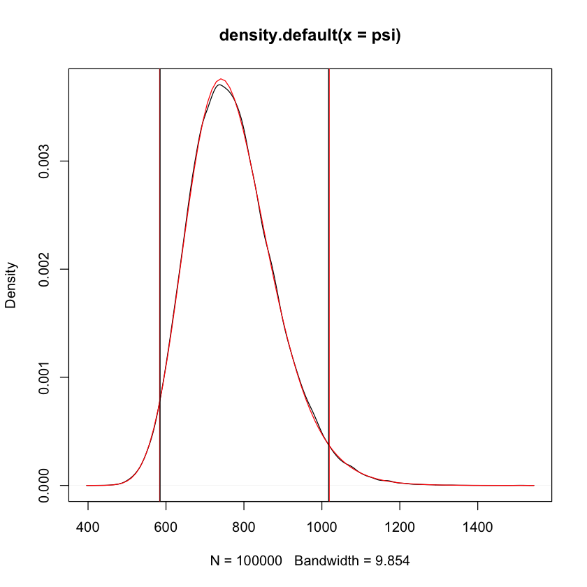
## 95% credible interval (quantile-based)
ci.exact=invgamma::qinvgamma(c(.025,.975),a,b)
ci.mc=quantile(psi,c(.025,.975))

# add intervals to posterior plot
plot(density(psi)) # kernel-density estimate
curve(invgamma::dinvgamma(x,a,b),add=TRUE,col=2)
abline(v=ci.exact,col=2)
abline(v=ci.mc)


## P( psi < 600 | data )
invgamma::pinvgamma(600,a,b)
mean(psi<600)


## MC error decreases slowly for large K
plot(cumsum(psi)/(1:K),xlim=c(1,10000),type='l',
     xlab='K',ylab='MC mean based on K samples')
abline(h=b/(a-1),col='red')



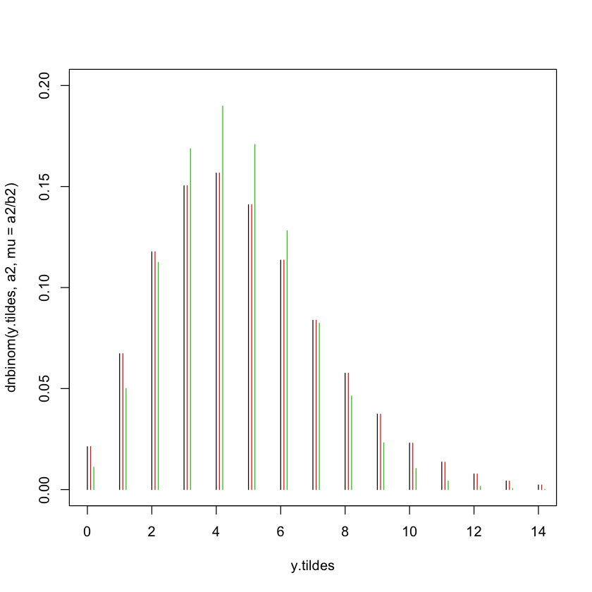
######   MC for predictive distribution in Poisson-gamma model

## assumed parameters
a=0.5; b=0 # jeffreys prior
y=c(5,4) # poisson observations

## posterior of mean parameter theta
n=length(y)
a2=a+sum(y)
b2=b+n
curve(dgamma(x,a2,b2),0,2.5*mean(y))


## exact posterior predictive distributions
y.tildes=0:round(3*mean(y))
plot(y.tildes,dnbinom(y.tildes,a2,mu=a2/b2),ylim=c(0,.2),type='h')

## MC approximation of post. pred. distr.
thetas=rgamma(K,a2,b2) # sample from posterior
pp.mc=numeric(length=length(y.tildes))
for(j in 1:length(pp.mc)) pp.mc[j]=mean(dpois(y.tildes[j],thetas))
lines(y.tildes+1e-1,pp.mc,type='h',col=2)

## predictive distribution, plugging in MLE
lines(y.tildes+2e-1,dpois(y.tildes,mean(y)),type='h',col=3)




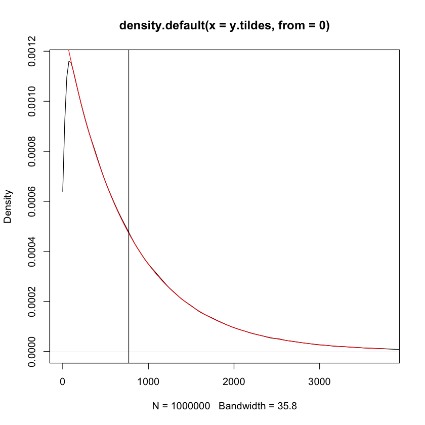
#### posterior predictive distribution for exponential-gamma model

K=1e6

## parameters of the posterior of the rate parameter
a=50
b=37815

## posterior draws of the rate parameter
thetas=rgamma(K,a,rate=b)

## MC samples from post. pred. distr.
y.tildes=rexp(K,thetas)

## MC (kernel density) estimate of posterior pred
plot(density(y.tildes,from=0),xlim=c(0,5*b/a))

## exact posterior pred
curve(a*b^a/(x+b)^(a+1),add=TRUE,col=2)

## MC estimate of PP mean
mean.pp=mean(y.tildes)
mean.pp # exact mean: 771.7
abline(v=mean.pp)

771.734693877551

771.831659052567

111.390308313294

111.218024621904

0.0401536510132767

0.03917

770.948738931396